Linear Algebra Made Efficient: Strassen Matrix Multiplication

In college, you’ve probably encountered linear algebra and learned about matrix multiplication. You may have implemented a matrix multiplication algorithm using nested for loops, which has a time complexity of \(O(n^3)\). In this blog post, we’ll explore the Strassen algorithm, an efficient method for multiplying large matrices.

Traditional Matrix Multiplication

Matrix multiplication involves nested loops that iterate through the dimensions of two matrices. This results in a time complexity of \(O(n^3)\), which can be computationally expensive for large matrices. Here’s a Python implementation of traditional matrix multiplication:

def mul_matrix(X, Y):
  Z = [[0 for i in range(len(X))] for j in range(len(Y))]
  for i in range(len(X)):
    for j in range(len(Y[0])):
      for k in range(len(X[0])):
        Z[i][j] += X[i][k] * Y[k][j]
  return Z

The Strassen Algorithm

Volker Strassen devised a more efficient algorithm for multiplying large matrices, provided they are squared and have dimensions that are powers of two. The Strassen algorithm breaks down matrix multiplication into smaller subproblems, reducing the overall complexity.

For more information about the Strassen algorithm, check out this Wikipedia article.

The Process

Let \(X\), \(Y\) two squared matrices and \(Z\) the product of those matrices. If \(X\) and \(Y\) do not have the shape \(2^n \times 2^n\) (that is to say, their shape is not of power of two) will have to fill those empty spaces with zeros.

Let’s start with chunks of the same size.

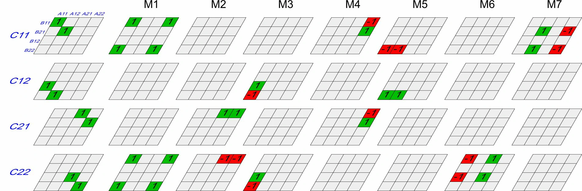
\[X=\begin{pmatrix} A & B\\ C & D \end{pmatrix}, Y=\begin{pmatrix} E & F\\ G & H \end{pmatrix}, Z=\begin{pmatrix} Z_{11} & Z_{12}\\ Z_{21} & Z_{22} \end{pmatrix}\]

It is worth say that \(A\), \(B\), \(C\), \(D\), \(E\), \(F\), \(G\), \(H\) and \(Z_{ij}\) follow the requirements of Strassen algorithm. Then, multiplying \(X\) and \(Y\) we get:

\[Z_{11} = AE+BG\] \[Z_{12} = AF+BH\] \[Z_{21} = CE+DG\] \[Z_{22} = CF+DH\]

With this the number of multiplications does not reduce. But if we define the following matrices:

\[P_{1} = A(F-H)\] \[P_{2} = (A+B)H\] \[P_{3} = (C+D)E\] \[P_{4} = D(G-E)\] \[P_{5} = (A+D)(E+H)\] \[P_{6} = (B-D)(G+H)\] \[P_{7} = (A-C)(E+F)\]

We can rewrite \(Z\) as follows:

\[Z=\begin{pmatrix} P_{5}+P_{4}-P_{2}+P_{6} & P_{1}+P_{2}\\ P_{3} + P_{4} & P_{5}+P_{1}-P_{3}-P_{7} \end{pmatrix}\]

This process should be repeated recursively until we get a \(2 \times 2\) matrix.

Python Implementation

To understand better this process let’s implement this algorithm in Python. We need auxiliary functions which allows us to divide the matrices and merge them.

Divide Matrices

def divide_matrix(A):
  mid = len(A)//2
  m_11 = [M[:mid] for M in A[:mid]]
  m_12 = [M[mid:] for M in A[:mid]]
  m_21 = [M[:mid] for M in A[mid:]]
  m_22 = [M[mid:] for M in A[mid:]]

  return (m_11, m_12, m_21, m_22)

Merge Matrices

def merge_matrix(matrix_11, matrix_12, matrix_21, matrix_22):
  matrix_total = []
  rows1 = len(matrix_11)
  rows2 = len(matrix_21)
  for i in range(rows1):
    matrix_total.append(matrix_11[i] + matrix_12[i])
  for j in range(rows2):
    matrix_total.append(matrix_21[j] + matrix_22[j])
  return matrix_total

Add Matrices

def add_matrix(X, Y):
  n = len(X)
  if n == 1:
    return [[X[0][0] + Y[0][0]]]
  S = []
  for i in range(n):
    S.append([])
    for j in range(n):
      S[i].append(X[i][j] + Y[i][j])
  return S

Subtract Matrices

def sub_matrix(X, Y):
  n = len(X)
  if n == 1:
    return [[X[0][0] - Y[0][0]]]
  S = []
  for i in range(n):
    S.append([])
    for j in range(n):
      S[i].append(X[i][j] - Y[i][j])
  return S

Algorithm Implementation

Finally, we can implement the Strassen algorithm as explained before. Notice that it always use Strassen for multiplying the submatrices, so it is recursive.

def strassen(X, Y):
  if len(X) == 1:
    return [[X[0][0] * Y[0][0]]]
  else:
    A, B, C, D = divide_matrix(X)
    E, F, G, H = divide_matrix(Y)
    
    P1 = strassen(A, sub_matrix(F,H))
    P2 = strassen(add_matrix(A, B), H)
    P3 = strassen(add_matrix(C, D), E)
    P4 = strassen(D, sub_matrix(G, E))
    P5 = strassen(add_matrix(A, D), add_matrix(E, H))
    P6 = strassen(sub_matrix(B, D), add_matrix(G, H))
    P7 = strassen(sub_matrix(A, C), add_matrix(E, F))
    
    Z11 = add_matrix(sub_matrix(add_matrix(P5, P4), P2), P6)
    Z12 = add_matrix(P1, P2)
    Z21 = add_matrix(P3, P4)
    Z22 = sub_matrix(sub_matrix(add_matrix(P5, P1), P3), P7)

    return merge_matrix(Z11, Z12, Z21, Z22)

You can test it like this:

A = [[1,2,3,4],[5,6,7,8],[9,10,11,12],[13,14,15,16]]
B = [[1,1,1,1],[1,1,1,1],[1,1,1,1],[1,1,1,0]]

print("Strassen")
print(*strassen(A,B), sep='\n')
print("\nClassic")
print(*mul_matrix(A,B), sep='\n')

Output:

\[\begin{pmatrix} 1 & 2 & 3 & 4\\ 5 & 6 & 7 & 8\\ 9 & 10 & 11 & 12\\ 13 & 14 & 15 & 16 \end{pmatrix} \begin{pmatrix} 1 & 1 & 1 & 1\\ 1 & 1 & 1 & 1\\ 1 & 1 & 1 & 1\\ 1 & 1 & 1 & 0 \end{pmatrix} =\begin{pmatrix} 10& 10& 10& 6\\ 26& 26& 26& 18\\ 42& 42& 42& 30\\ 58& 58& 58& 42 \end{pmatrix}\]

Conclusion

The upper bound of the classic method is \(O(n^3)\). But for the Strassen algorithm it is \(O(n^{\log_{2}7})\) or about \(O(n^{2.807})\). Maybe you will say that the difference is just a few decimals, but with the next plot you will realize that the difference is important. The complexity of the classic version grows faster as \(n\) increases.

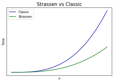Classic method Vs. Strassen comparison

You can find the complete Python code for the Strassen algorithm here. Feel free to leave comments, questions, or follow me on social media for more content like this.