Karatsuba's Algorithm in Python: Multiplying Large Numbers Efficiently

Multiplying numbers is a fundamental mathematical operation, and we all learn various methods for doing so in school. However, when it comes to dealing with large numbers, this seemingly simple task can become quite computationally expensive. In such scenarios, we need smarter algorithms to optimize the process. Anatoly Karatsuba’s algorithm offers a brilliant solution that, while complex for humans, is incredibly efficient for computers.

The Divide and Conquer Approach

Karatsuba’s algorithm is a classic example of a divide-and-conquer approach to multiplication. It simplifies a multiplication operation into smaller multiplications with some additions. By breaking down the problem, it reduces the time complexity, even if it requires three multiplications. Notably, these multiplications involve smaller numbers.

Let’s assume we want to multiply two numbers, x and y. We can represent these numbers in a different base:

\[x = x_1 B^m + x_0\] \[y = y_1 B^m + y_0\]

For the sake of human understanding, we’ll consider B to be 10, as we use the decimal system. Expanding the expression, we get:

\[xy = (x_1\times 10^m + x_0)(y_1\times 10^m + y_0)\\\]

Let’s expand the expression:

\[xy = x_1y_1\times 10^{2m}+(x_1y_0+x_0y_1)\times 10^m+x_0y_0\]

Now, let’s define some intermediate variables:

\[r = x_1y_1\] \[s = x_0y_0\] \[t = x_1y_0+x_0y_1\]

With a bit of mathematical manipulation, we can express t based on r and s to reduce one multiplication:

\[x_1y_0+x_0y_1=x_1y_0+x_1y_1+x_0y_0-x_1y_1-x_0y_0+x_0y_1\]

We can express \(t\) based on \(r\) and \(s\) to reduce one multiplication.

\[t=(x_1+x_0)(y_1+y_0)-r-s\]

The final multiplication can be expressed as:

\[xy=r\times 10^{2m}+t\times 10^m+s\]

Example

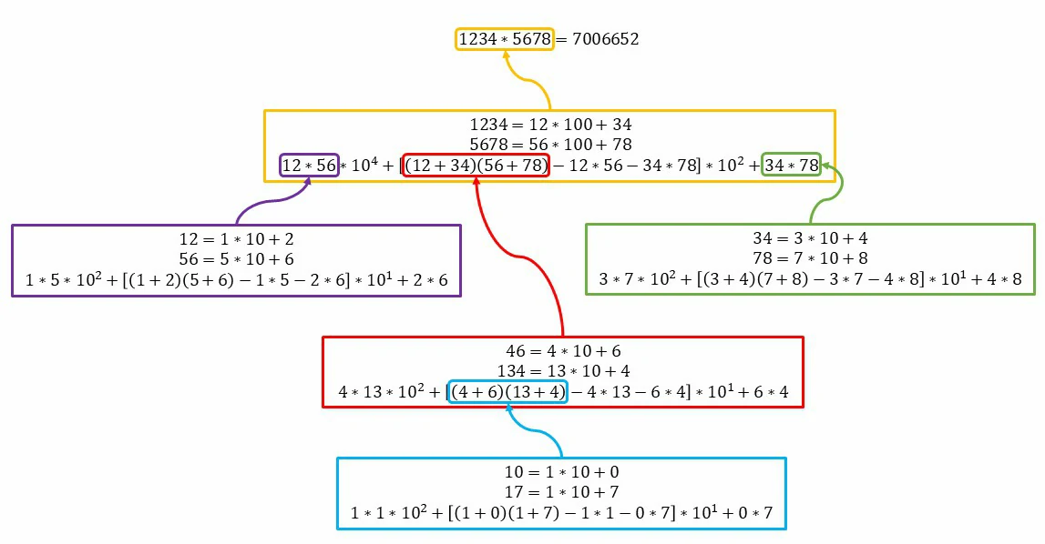
To visualize how this algorithm works, take a look at the following illustration:

---
title: Karatsuba's Algorithm Functionality
---
flowchart TD
    A[1234*5678 = 7006652] --> B[1234 = 12*100 + 34]
    A --> C[5678 = 56 * 100 + 78]
    C --> D["12*56 * 10^4 + [(12+34)(56+78) - 12*56 - 34*78] * 10^2 + 34*78"]
    B --> D
    D --> E["12*56"]
    D --> I["34*78"]
    D --> H["(12+34)(56+78)"]
    E --> F["12 = 1*10 + 2"]
    E --> G["56 = 5*10 + 6"]
    F --> K["1*5 * 10^2 + [(1+2)(5+6) - 1*5 - 2*6] * 10^1 + 2*6"]
    G --> K
    I --> L["34 = 3*10 + 4"]
    I --> M["78 = 7*10 + 8"]
    M --> N["3*7 * 10^2 + [(3+4)(7+8) - 3*7 - 4*8] * 10^1 + 4*8"]
    L --> N
    H --> O["46 = 4*10 + 6"]
    H --> P["134 = 13*10 + 4"]
    O --> Q["4*13 * 10^2 + [(4+6)(13+4) - 4*13 - 6*4] * 10^1 + 6*4"]
    P --> Q
    Q --> R["(4+6)(13+4)"]
    R --> T["10 = 1*10 + 0"]
    R --> U["17 = 1*10 + 7"]
    T --> V["1*1 * 10^2 + [(1+0)(1+7) - 1*1 - 0*7] * 10^1 + 0*7"]
    U --> V

Python Implementation

We can clearly see that we’ve reduced the number of multiplications to three. Now, let’s implement this in Python.

def karatsuba(x: int, y: int) -> int:
    if x < 10:
        return x * y
    else:
        if x > y:
            x, y = y, x

        m = len(str(x))//2

        x1, x0 = divmod(x, 10**m)
        y1, y0 = divmod(y, 10**m)

        r = karatsuba(x1, y1)
        s = karatsuba(x0, y0)

        t = karatsuba(x1+x0, y1+y0) - r - s

        return r*10**2*m + t*10**m + s

It’s important to note that the primary goal here is to understand the algorithm’s functionality, rather than using it in real-world projects. In practice, many of these optimizations are already implemented at a low level, often in the hardware itself.

I hope this post has been helpful in shedding light on the fascinating world of efficient multiplication algorithms. If you have any questions or comments, please feel free to reach out. For more content like this, follow me on social media.